3 ANN in R
3.1 Step 1: Collecting data
For this analysis, we will utilize data on the compressive strength of concrete donated to the UCI Machine Learning Data Repository (http://archive.ics.uci.edu/ml) by I-Cheng Yeh. As he found success using neural networks to model these data, we will attempt to replicate his work using a simple neural network model in R.
According to the website, the concrete dataset contains 1,030 examples of concrete with eight features describing the components used in the mixture. These features are thought to be related to the final compressive strength and they include the amount (in kilograms per cubic meter) of cement, slag, ash, water, superplasticizer,coarse aggregate, and fine aggregate used in the product in addition to the aging time (measured in days).
3.2 Step 2: Exploring and preparing the data
Read in data and examine structure.
Download the file from here and save it in a folder named data in your working directory.
concrete <- readxl::read_excel("data/Concrete_Data.xlsx")
colnames(concrete) <- c('cement', 'slag', 'ash', 'water', 'superplastic', 'coarseagg', 'fineagg', 'age', 'strength')
str(concrete)
## tibble [1,030 × 9] (S3: tbl_df/tbl/data.frame)
##  $ cement      : num [1:1030] 540 540 332 332 199 ...
##  $ slag        : num [1:1030] 0 0 142 142 132 ...
##  $ ash         : num [1:1030] 0 0 0 0 0 0 0 0 0 0 ...
##  $ water       : num [1:1030] 162 162 228 228 192 228 228 228 228 228 ...
##  $ superplastic: num [1:1030] 2.5 2.5 0 0 0 0 0 0 0 0 ...
##  $ coarseagg   : num [1:1030] 1040 1055 932 932 978 ...
##  $ fineagg     : num [1:1030] 676 676 594 594 826 ...
##  $ age         : num [1:1030] 28 28 270 365 360 90 365 28 28 28 ...
##  $ strength    : num [1:1030] 80 61.9 40.3 41.1 44.3 ...
Custom normalization function:
Neural networks work best when the input data are scaled to a narrow range around zero, and here,we see values ranging anywhere from zero up to over a thousand.Therefore, we apply normalization to entire data frame:
Confirm that the range is now between zero and one:
summary(concrete_norm$strength)
##    Min. 1st Qu.  Median    Mean 3rd Qu.    Max.
##  0.0000  0.2663  0.4000  0.4172  0.5457  1.0000
Compared to the original minimum and maximum:
summary(concrete$strength)
##    Min. 1st Qu.  Median    Mean 3rd Qu.    Max.
##   2.332  23.707  34.443  35.818  46.136  82.599
Create training and test data:
3.3 Step 3: Training a model on the data
Train the neuralnet model: (another package is ‘nnet’)
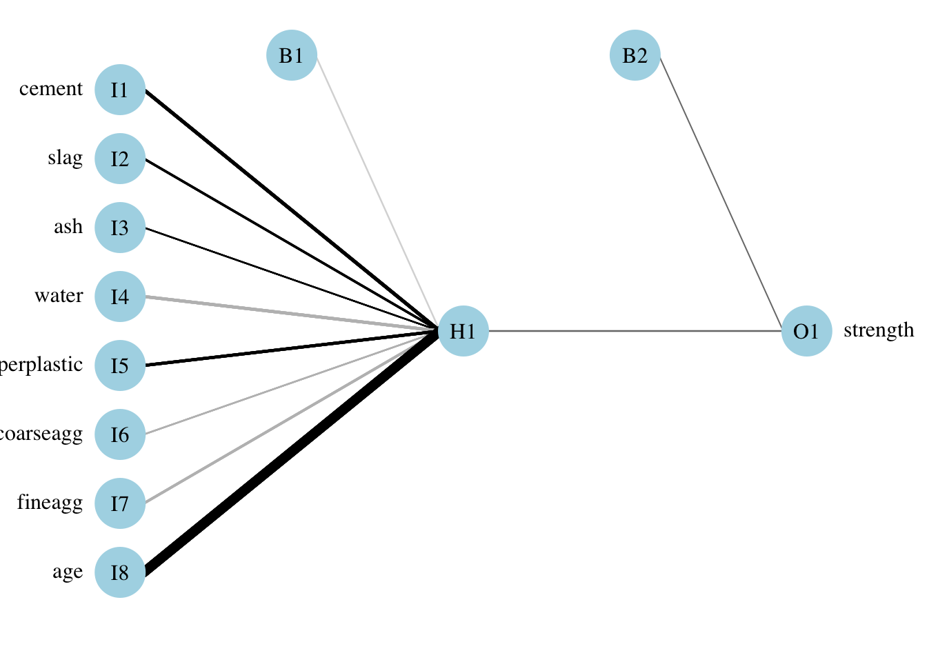
Simple ANN with only a single hidden neuron:
set.seed(12345) # to guarantee repeatable results
concrete_model <- neuralnet(formula = strength ~ cement + slag +
                              ash + water + superplastic +
                              coarseagg + fineagg + age,
                            data = concrete_train)
Visualize the network topology:
Alternative plot:
Plotnet:
3.4 Step 4: Evaluating model performance
Obtain model results:
Obtain predicted strength values:
Examine the correlation between predicted and actual values:
cor(predicted_strength, concrete_test$strength)   # higher than stated in book 0.7170368646
##           [,1]
## [1,] 0.7196329
Produce actual predictions by:
head(predicted_strength)
##          [,1]
## 774 0.3900450
## 775 0.2423273
## 776 0.2503669
## 777 0.2276142
## 778 0.3321605
## 779 0.1832346

concrete_train_original_strength <- concrete[1:773,"strength"]

strength_min <- min(concrete_train_original_strength)
strength_max <- max(concrete_train_original_strength)

head(concrete_train_original_strength)
## # A tibble: 6 x 1
##   strength
##      <dbl>
## 1     80.0
## 2     61.9
## 3     40.3
## 4     41.1
## 5     44.3
## 6     47.0
Custom normalization function:
3.5 Step 5: Improving model performance
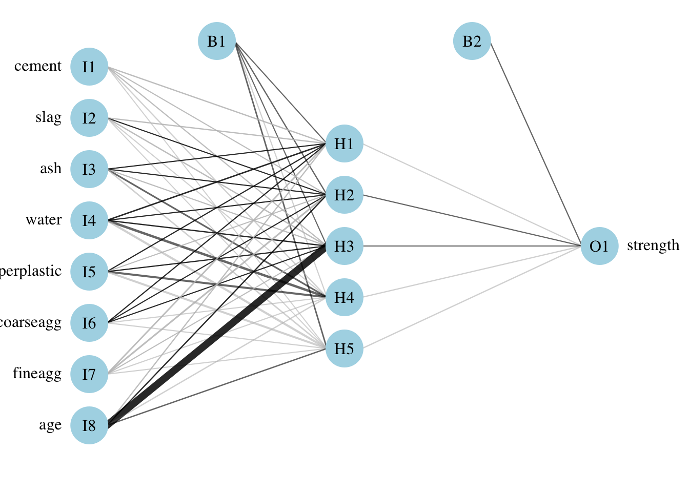
A more complex neural network topology with 5 hidden neurons:
set.seed(12345) # to guarantee repeatable results
concrete_model2 <- neuralnet(strength ~ cement + slag +
                               ash + water + superplastic +
                               coarseagg + fineagg + age,
                             data = concrete_train, hidden = 5, act.fct = "logistic")
Plot the network:
Plotnet:
Evaluate the results as we did before:
model_results2 <- compute(concrete_model2, concrete_test[1:8])
predicted_strength2 <- model_results2$net.result
cor(predicted_strength2, concrete_test$strength)
##           [,1]
## [1,] 0.7814216
Try different activation function: A more complex neural network topology with 5 hidden neurons: (Change to hidden = 3, the correlation is almost the same as 5)
set.seed(12345) # to guarantee repeatable results
concrete_model2 <- neuralnet(strength ~ cement + slag +
                               ash + water + superplastic +
                               coarseagg + fineagg + age,
                             data = concrete_train, hidden = 5, act.fct = "tanh")
Evaluate the results as we did before: