3 DIMENSIONALITY REDUCTION IN R
Since we are not trying to predict the value of any target variable like in supervised approaches, the value of unsupervised machine learning can be to see how data can be separated based solely on the nature of their features. This is of major value, as we can include all of the data at once, and just see how it sorts! Unsupervised approaches are also useful for optimizing other machine learning algorithms.
Principal component analysis (PCA) is a powerful linear transformation technique used to explore patterns in data and highly correlated variables. It is useful for distilling variation across many variables onto a reduced feature space, such as a two-dimensional scatterplot.
3.1 Reclass variables
dplyr is essential for changing the classes of multiple features at once :^)
3.3 Scale numeric variables
vars_to_scale = c("age", "trestbps", "chol", "thalach", "oldpeak")
h = data_original %>% mutate_at(scale, .vars = vars(vars_to_scale))
## Note: Using an external vector in selections is ambiguous.
## ℹ Use `all_of(vars_to_scale)` instead of `vars_to_scale` to silence this message.
## ℹ See <https://tidyselect.r-lib.org/reference/faq-external-vector.html>.
## This message is displayed once per session.## age sex cp trestbps chol fbs restecg thalach exang
## 1 0.9506240 1 3 0.76269408 -0.25591036 1 0 0.01541728 0
## 2 -1.9121497 1 2 -0.09258463 0.07208025 0 1 1.63077374 0
## 3 -1.4717230 0 1 -0.09258463 -0.81542377 0 0 0.97589950 0
## 4 0.1798773 1 1 -0.66277043 -0.19802967 0 1 1.23784920 0
## 5 0.2899839 0 0 -0.66277043 2.07861109 0 1 0.58297496 1
## 6 0.2899839 1 0 0.47760118 -1.04694656 0 1 -0.07189928 0
## oldpeak slope ca thal target
## 1 1.0855423 0 0 1 1
## 2 2.1190672 0 0 2 1
## 3 0.3103986 2 0 2 1
## 4 -0.2063639 2 0 2 1
## 5 -0.3786180 2 0 2 1
## 6 -0.5508722 1 0 1 13.4 Factorize categorical variables
# Quick rename target outcomes
h$target = ifelse(h$target == 1, "yes", "no")

vars_to_fac = c("sex", "cp", "fbs", "restecg", "exang",
                "slope", "ca", "thal", "target")

h = h %>% mutate_at(as.factor, .vars = vars(vars_to_fac))
## Note: Using an external vector in selections is ambiguous.
## ℹ Use `all_of(vars_to_fac)` instead of `vars_to_fac` to silence this message.
## ℹ See <https://tidyselect.r-lib.org/reference/faq-external-vector.html>.
## This message is displayed once per session.## age sex cp trestbps chol fbs restecg thalach
## "numeric" "factor" "factor" "numeric" "numeric" "factor" "factor" "numeric"
## exang oldpeak slope ca thal target
## "factor" "numeric" "factor" "factor" "factor" "factor"# Create subset of numeric-only data (along with h.target)
# Combine the scaled numeric data and the original target feature
ml_num = data.frame(subset(h, select = vars_to_scale), h$target)
head(ml_num)## age trestbps chol thalach oldpeak h.target
## 1 0.9506240 0.76269408 -0.25591036 0.01541728 1.0855423 yes
## 2 -1.9121497 -0.09258463 0.07208025 1.63077374 2.1190672 yes
## 3 -1.4717230 -0.09258463 -0.81542377 0.97589950 0.3103986 yes
## 4 0.1798773 -0.66277043 -0.19802967 1.23784920 -0.2063639 yes
## 5 0.2899839 -0.66277043 2.07861109 0.58297496 -0.3786180 yes
## 6 0.2899839 0.47760118 -1.04694656 -0.07189928 -0.5508722 yes3.5 Fit model
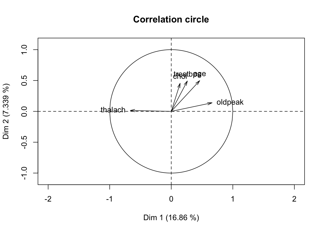
split = splitmix(h)
X1 = split$X.quanti
X2 = split$X.quali
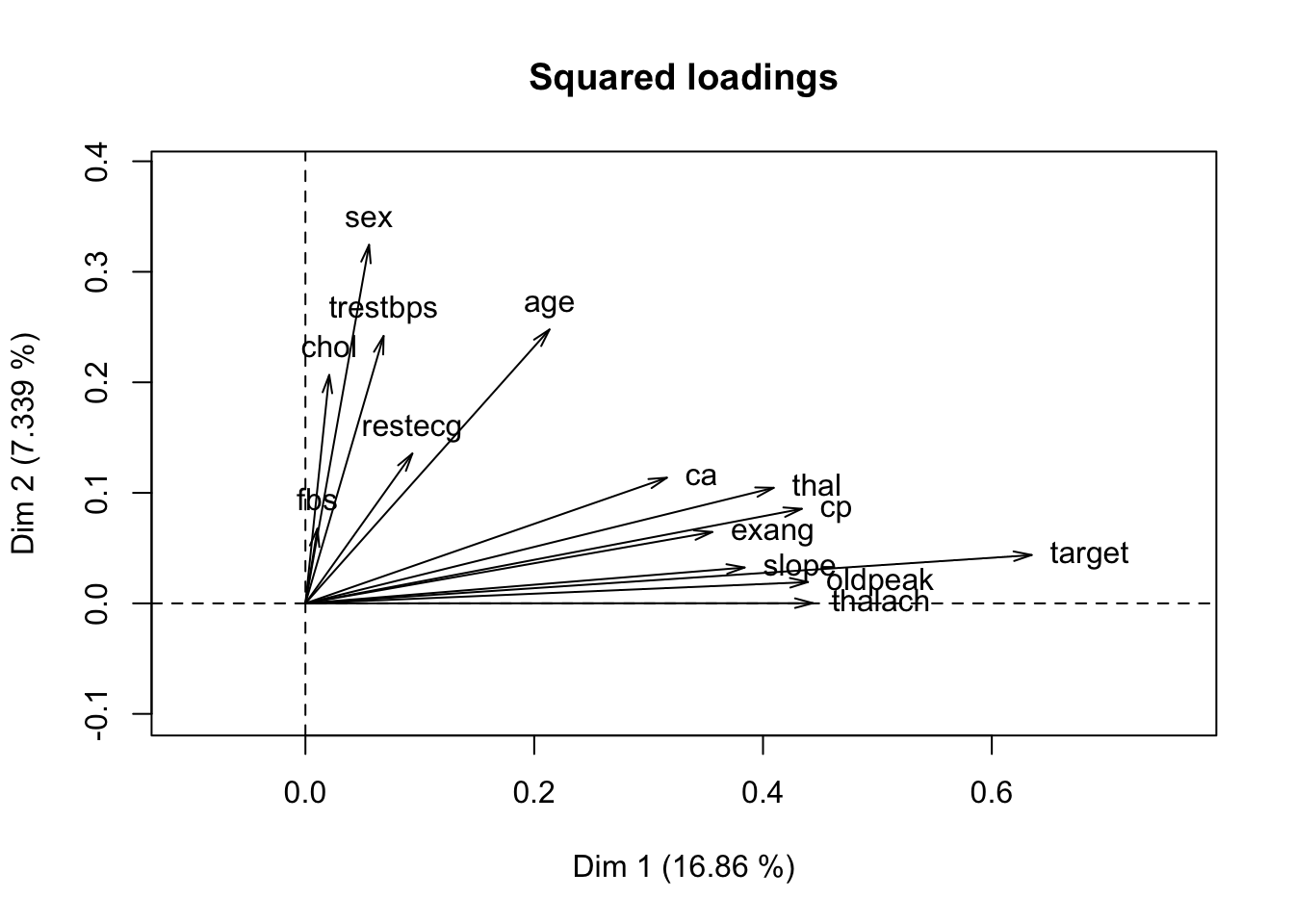
res.pcamix = PCAmix(X.quanti = X1,
X.quali = X2,
rename.level = TRUE,
graph = TRUE)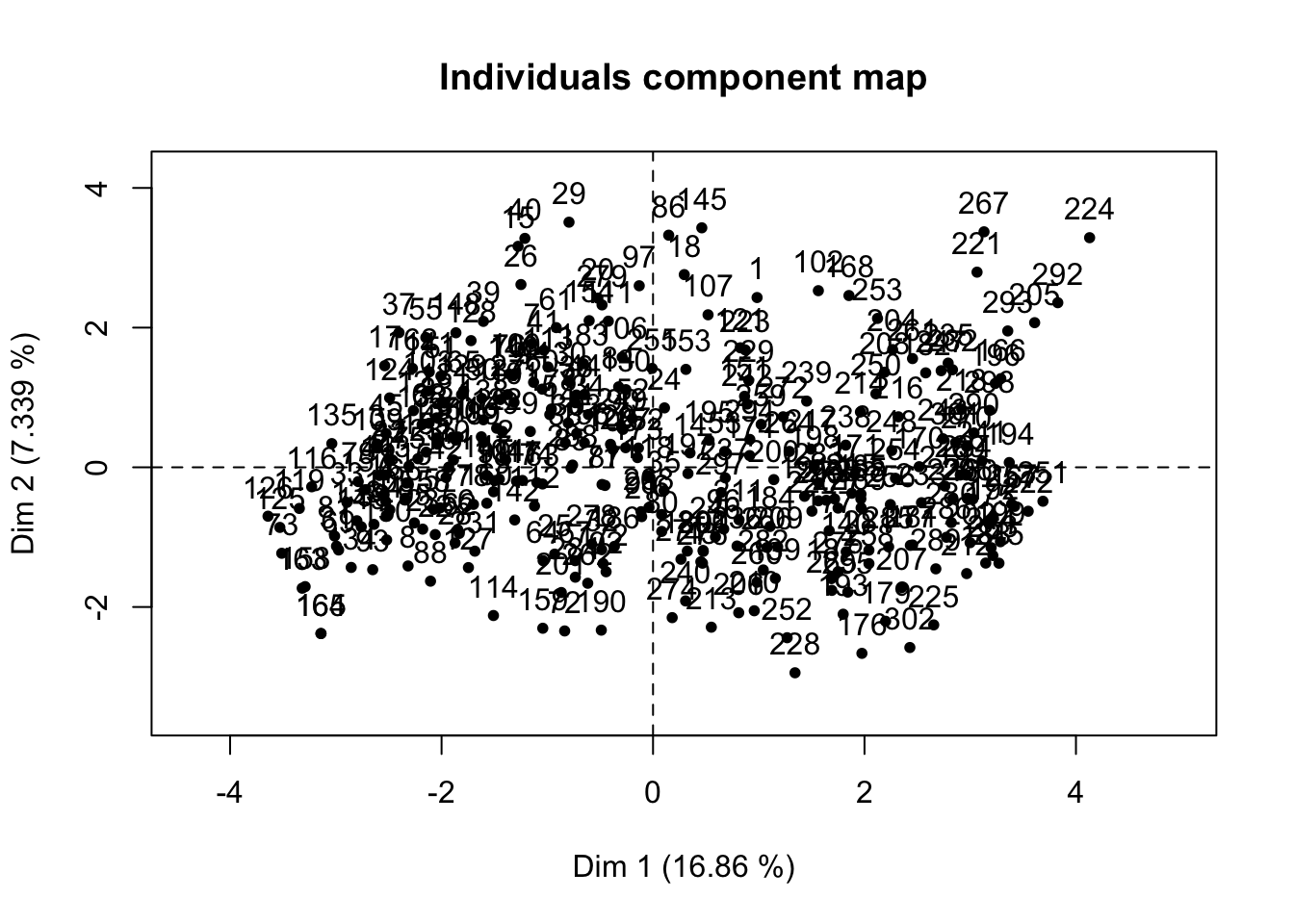
##  [1] "call"         "eig"          "ind"          "quanti"       "levels"
##  [6] "quali"        "sqload"       "coef"         "Z"            "M"
## [11] "quanti.sup"   "levels.sup"   "sqload.sup"   "rec.sup"      "scores.stand"
## [16] "scores"       "V"            "A"            "categ.coord"  "quanti.cor"
## [21] "quali.eta2" "rec" "ndim" "W" "rename.level"## Eigenvalue Proportion Cumulative
## dim 1 3.8787886 16.864298 16.86430
## dim 2 1.6879338 7.338843 24.20314
## dim 3 1.4908837 6.482103 30.68524
## dim 4 1.3312321 5.787966 36.47321
## dim 5 1.2157241 5.285757 41.75897
## dim 6 1.1179188 4.860517 46.61948
## dim 7 1.0869543 4.725888 51.34537
## dim 8 1.0522819 4.575138 55.92051
## dim 9 1.0343524 4.497184 60.41769
## dim 10 0.9604933 4.176058 64.59375
## dim 11 0.9299643 4.043323 68.63707
## dim 12 0.8961699 3.896391 72.53347
## dim 13 0.8255254 3.589241 76.12271
## dim 14 0.8045898 3.498217 79.62092
## dim 15 0.7339800 3.191217 82.81214
## dim 16 0.7237726 3.146838 85.95898
## dim 17 0.6862958 2.983895 88.94287
## dim 18 0.5911739 2.570321 91.51319
## dim 19 0.5082960 2.209983 93.72318
## dim 20 0.4234490 1.841083 95.56426
## dim 21 0.3820072 1.660901 97.22516
## dim 22 0.3484562 1.515027 98.74019
## dim 23 0.2897568 1.259812 100.00000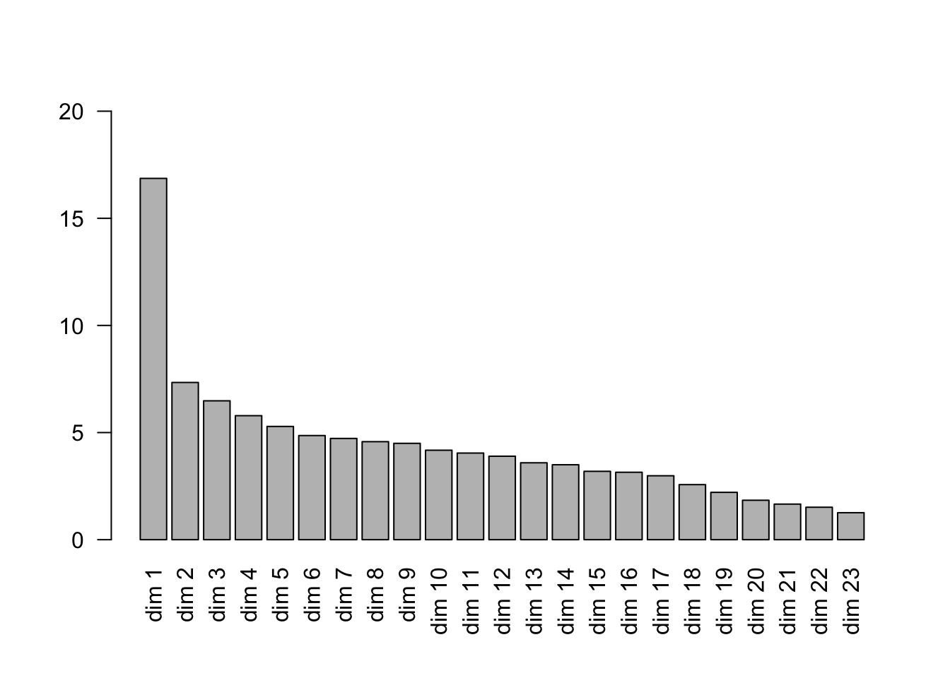
3.7 ggplot coordinates
# ?plot.PCAmix
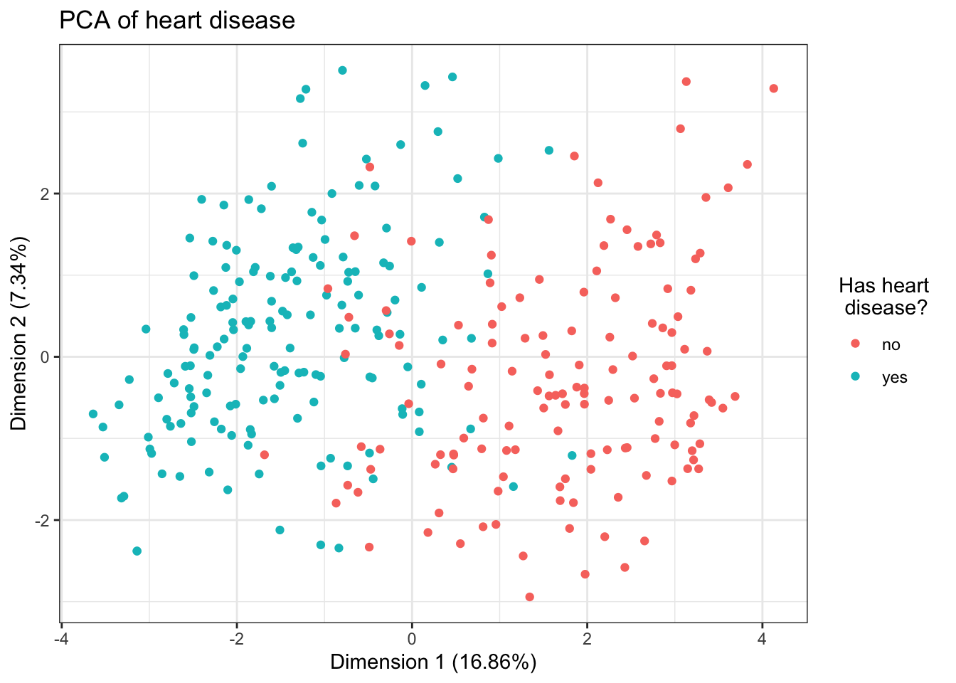
# Convert the coordinates to a dataframe, and add the original target column
pca1 = data.frame(res.pcamix$ind$coord, h$target)
ggplot(pca1, aes(x = dim.1, y = dim.2, color = h.target)) +
geom_point() +
theme_bw() +
guides(color = guide_legend(title = "Has heart \n disease?")) +
ggtitle("PCA of heart disease") +
xlab(paste("Dimension 1", paste0("(",
round(res.pcamix$eig[1, 2], 2),
"%", ")"))) +
ylab(paste("Dimension 2", paste0("(",
round(res.pcamix$eig[2, 2], 2),
"%", ")")))
3.8 View factor loadings
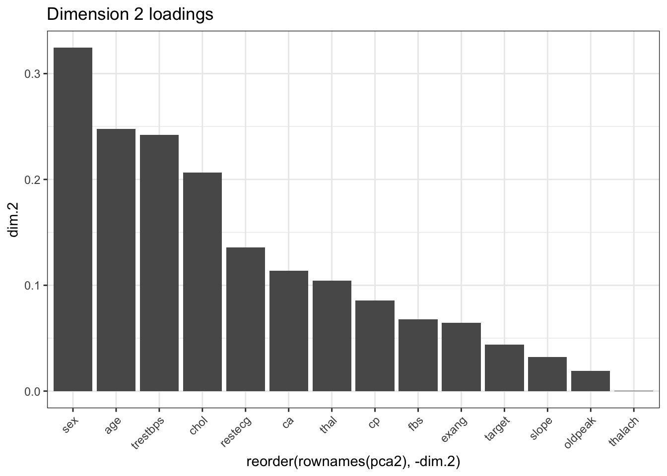
##               dim.1        dim.2       dim.3       dim.4       dim.5
## age      0.21337352 0.2477799674 0.041744496 0.031009752 0.034038015
## trestbps 0.06834390 0.2419102430 0.082816187 0.051728438 0.001589446
## chol     0.02082961 0.2066356059 0.152307150 0.043233560 0.049610585
## thalach  0.44360573 0.0002023463 0.047419425 0.058275497 0.046975232
## oldpeak  0.43930006 0.0193048486 0.082960245 0.086332841 0.025271527
## sex      0.05563966 0.3243727308 0.160043366 0.069228609 0.007629010
## cp       0.43389618 0.0855538209 0.231154112 0.046455629 0.376511477
## fbs      0.01052402 0.0676379198 0.110885644 0.133605806 0.178892828
## restecg  0.09350096 0.1355432393 0.002523635 0.325035267 0.007697222
## exang    0.35569689 0.0645725466 0.015438480 0.001024528 0.010754496
## slope    0.38393372 0.0324258579 0.318500790 0.183487912 0.019374687
## ca       0.31595887 0.1136921858 0.137120105 0.208372158 0.342211693
## thal     0.40934316 0.1045544271 0.104108768 0.073799024 0.112059111
## target   0.63484228 0.0437480745 0.003861254 0.019643099 0.003108742
# Dimension 1
ggplot(pca2, aes(x = reorder(rownames(pca2), -dim.1), y = dim.1)) +
geom_bar(stat = "identity") +
theme_bw() + ggtitle("Dimension 1 loadings") +
theme(axis.text.x = element_text(angle = 45, hjust = 1))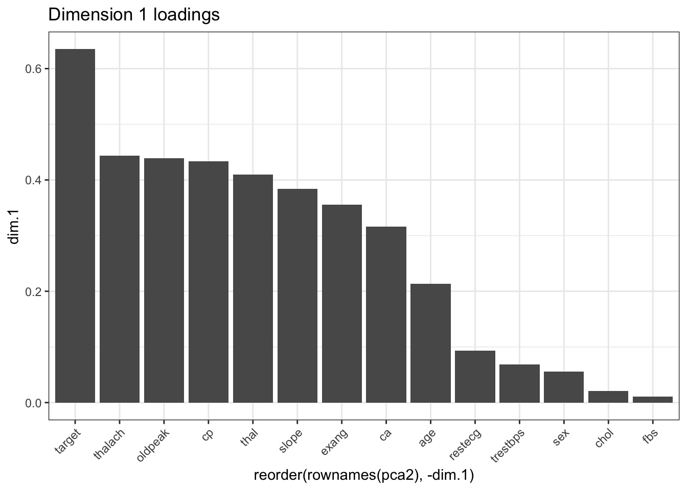
# Dimension 2
ggplot(pca2, aes(x = reorder(rownames(pca2), -dim.2), y = dim.2)) +
  geom_bar(stat = "identity") +
  theme_bw() + ggtitle("Dimension 2 loadings") +
  theme(axis.text.x = element_text(angle = 45, hjust = 1))