4 PCA FOR MACHINE LEARNING IN R
Create a 70/30 training/test split
# Set seed for reproducibility
set.seed(1)

# Create a stratified random split
training_rows = caret::createDataPartition(ml_num$h.target,
                                           p = 0.70, list = FALSE)

# Partition training dataset
train_x_class = ml_num[training_rows, ]

# Partition test dataset
test_x_class = ml_num[-training_rows, ]

dim(train_x_class)
## [1] 213 6## [1] 90 6##
## no yes
## 97 116##
## no yes
## 41 494.1 Fit PCA model to training set for numeric values
?prcomp
pca_ml = prcomp(subset(train_x_class, select = -h.target),
                       retx = TRUE,
                       center = FALSE, scale = FALSE)
pca_ml
## Standard deviations (1, .., p=5):
## [1] 1.3433029 1.0702577 1.0024705 0.8699753 0.7086122
##
## Rotation (n x k) = (5 x 5):
## PC1 PC2 PC3 PC4 PC5
## age 0.5518423 0.1059808 0.1358815 0.49852917 0.6459436
## trestbps 0.3295905 0.5611404 -0.7087114 0.05481389 -0.2668618
## chol 0.3127980 0.5539657 0.6586925 -0.30551601 -0.2608901
## thalach -0.5286582 0.5219200 -0.0809096 -0.28283066 0.6013156
## oldpeak 0.4577315 -0.3075892 -0.1970845 -0.75837384 0.2861776## Importance of components:
## PC1 PC2 PC3 PC4 PC5
## Standard deviation 1.3433 1.0703 1.0025 0.8700 0.70861
## Proportion of Variance 0.3461 0.2197 0.1928 0.1452 0.09631
## Cumulative Proportion 0.3461 0.5658 0.7585 0.9037 1.00000## [1] 34.6090 21.9694 19.2746 14.5163 9.63074.2 Generate predicted values of PCs for test dataset
predicted_values = predict(pca_ml,
                           newdata = subset(test_x_class, select = -h.target))
head(predicted_values)
## PC1 PC2 PC3 PC4 PC5
## 1 1.1846594 0.06110625 -0.7951150 -0.2337026 0.79720858
## 3 -1.4715750 -0.24577784 -0.8116120 -1.0010592 -0.03755396
## 7 0.5700275 0.80468713 0.2365695 -0.3770120 -0.09933266
## 8 -1.6961573 0.49353662 0.6212806 -0.3133308 -0.28781615
## 11 -0.0844052 0.37950489 -0.5000747 -0.1837164 0.19438368
## 19 -0.6521884 0.82777404 -1.0568587 -1.1352000 -0.417675464.3 Define plotting parameters
4.4 Store the scores inside of dataframes
# Assign the data into dataframes like before
gg_train = data.frame(pca_ml$x[, target_PCs])
head(gg_train)
## PC1 PC2
## 2 -0.9553317 -0.01534275
## 4 -0.9299807 0.24698821
## 5 0.1102680 1.23102981
## 6 -0.2241860 -0.14932181
## 9 -0.1680809 1.18351579
## 10 -0.3081090 0.18865942## PC1 PC2
## 1 1.1846594 0.06110625
## 3 -1.4715750 -0.24577784
## 7 0.5700275 0.80468713
## 8 -1.6961573 0.49353662
## 11 -0.0844052 0.37950489
## 19 -0.6521884 0.827774044.5 Visualize
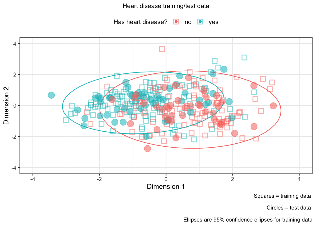
We can plot the training and test data on the same plot!
ggplot(
  # training data
  gg_train, aes(x = gg_train[,1], y = gg_train[,2],
                color = train_x_class$h.target)) +
  geom_point(shape = 0, alpha = .5, stroke = 1, size = 3) +
  stat_ellipse(show.legend = FALSE, lwd = 0.5) +
  labs(color = "Has heart disease?",
       caption = "Squares = training data \n
       Circles = test data \n
       Ellipses are 95% confidence ellipses for training data") +
  xlab("Dimension 1") +
  ylab("Dimension 2") +
  xlim(c(-4, 4)) +
  ylim(c(-4, 4)) +
  theme_bw() +

  # test data

  geom_point(gg_test, mapping = aes(x = gg_test[,1], y = gg_test[,2],
                                    color = test_x_class$h.target,
                                    size = 3, alpha = 0.75)) +
  guides(size = FALSE, alpha = FALSE) +
  theme(legend.position = "top") +
  ggtitle("Heart disease training/test data") +
  theme(plot.title = element_text(hjust = 0.5, size = 10),
        legend.title = element_text(size = 10),
        legend.text = element_text(size = 10))